Evolutionary Games and Ecosystems (9b)

Lotka-Volterra Equations: Its Workings - 2

Competitor Population as Function of Aggression Intensity

Skip this one again, you equation-averse folks!
We apply the arguments of last chapter to the case of two competing species, whse dynamics is described by

　　　　　dx/dt = b x - a x² - R x y
　　　　　dy/dt = d y - c y² - S x y .

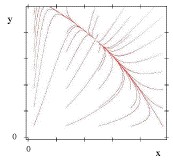
Solution to this problem does have stabel fixed point (X, Y) if R and S are sufficiently small as is shown in the phase diagram in the graph at the right. We now assume that species X controls R, and species Y controls S to their respective advantage. Since we have dX/dt=0, dy/dt = 0 , the function X[R,S] and Y[R,S] are determined from 　　　　　0 = b - a X[R,S] - R Y[R,S] 　　　　　0 = d - c Y[R,S] - S X[R,S]

Population of Competitors who are under a Common Predator

We now consider the case where both competitors have a common predator Z.

　　　　　dx/dt = b x - a x² - R x y - U x z
　　　　　dy/dt = d y - c y² - S x y - V y z
　　　　　dz/dt = -h z +f U x z + f V y z

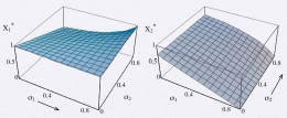
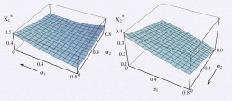
it is natural to assume that, at the fixed point (X、Y、Z) all species tweek with their own aggressive intensity ( X with R, Y with S and Z with V and U ). First optimize Z[V,U] with

　　　　dZ[U,V]/dU |_U*,V* =dZ[U,V]/dV |_U*,V* = 0

to obtain adiabatic expressions U*= U*(R,S) and V*= V*(R,S). Inserting these into the expression for x and Y gives us X[R,S] and Y[R,S] in the end. Right side of the graph above is an example of the plots X and Y as functions of both S and R. We observe that, in this case, X gains by decreasing R, and Y gains by decreasing S. The result is the pacification of both species X and Y who are stabiled at the stable fixed point as low aggression.