Discrete Models of Traffic Flow (2-1)

Fundametal Diagram and Flow Graph 1

Fundamental Diagram

If you can form intuitive images of the three concepts "density", "average velocity" and "flux" and understand the basic relation among them (1.1), an assurance can be given to you that you have already climbed the first wall surrounding the traffic flow model.

There are other quantities that could affect the traffic flow. Among them are the speed limit, the location and the properties of traffic signals, curvature and inclination of road segments, the status of pavements. These are the quantities outside of drivers' control, and simply given to them as an environment for driving. We call thse quantities "environmental parameters of traffic", or "traffic parameters" in short. A set of given parameter defines a road with a given condition.

As opposed to traffic parameters, the density of a traffic reflects the will of drivers who either decide to turn up on the road or stay home. The problem of traffic could be posed as the question of what the result of the decisions of drivers is in terms of traffic flow, whether a smooth free traffic is observed, or a traffic jam results. Since the degree of traffic jam is judged by average velocity or flux of the traffic, we can summarize the procedure of studying the traffic flow as follows:

In terms of an equation, this procedure is expressed as examing the flux F(\rho) or average velocity V(\rho) as functions of the density \rho. This of course does not imply the existense of any analytical relation, less in elementary functions.

We can always numerically obtain F or V for a given \rho. Graphical representation of \rho-V (or \rho-F) relation is achieved if we plot \rho in horizontal and V (or F) in vertical axis to obtain a two dimensional graph. The \rho vs. F plot is usually referred to as fundamental diagram of traffic flow We show, in the right, an example of a fundamental diagram. This shows three distinct behavior at low, intermediate and high \rho regions.

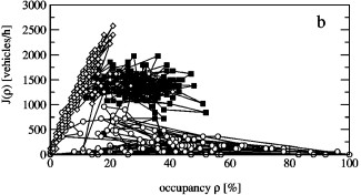
data taken from W. Knospe, et. al., Phys. Rev. E65 (2001) 015101(4)