Discrete Models of Traffic Flow (4-3)

Standard Model of Nagel and Schreckenberg 3

We look at the flow diagram to see how traffic develops in time for the case of R = 0. Four examples of different density with the maximum velocity U = 4 are shown.

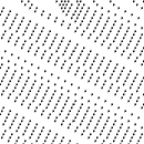	\rho=0.15	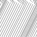\rho=0.25
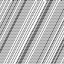	\rho=0.50	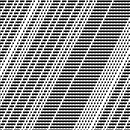\rho=0.75

The free traffic at the low density is represented here as lines flowing from top-left to bottom-right. At higher denity, the start of the traffic jam is signified by backward movement of the tail of jamming blocks which recedes with unit velocity

Above the critical density, the jamming block become dense, and is seen as dark texture on the flow diagram. With increasing \rho, the area occupied by the jamming bock becomes bigger.

Apart from the early stage of short transition from the initial configuration, the diagram appear quite "regular". This is true both for free traffic at low density such as \rho = 0.15 and for jammed traffic at high density such as \rho = 0.75. Once the pattern of the traffic is stabilized, it repeats itself with changing location and changing individual cars. The traffic flow for R = 0 is a typical example of the behavior of type II cellular automata.