Phase Structure of Segment Dependent NCS Model 3
In order to understand this rather puzzling fundamental diagram, we look into the flow diagram.
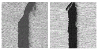
| In the flow diagram on the right, two traffic patterns under the same environmental parameters and the same denity, but staring from different initial conditions are dipicted. The parameters are the common maximum velocity U = 8, segment sizes L1 = 160 and L2 = 40. with non acceleration rates R1 = 0.1 and R2 = 0.4 respectively. The jamming block develops at the region of L2. |
|
The apparent difference in the colors of jamming blocks in the right and left diagrams reflects the different densities of the blocks as has been observed before. In this example, the dark jamming block of right hand graph is a block of absolute jamm with neighboring distance one and zero velocity, while the ligher jamming block of left hand side graph is a slow-moving jamm with neighboring distance two and the velocity one. Other types of lighter blocks with velocity two, and three can be also observed in other examples.
If there appears a jamming block with neighboring distance (W+1) in which cars advance with velocity W, and it takes hold with stability, that block limits the flux to the value FW = W / (W + 1). This explains the "quantization" (6.3). All of the jamming blocks are meta stable. The fluctuation is the result of the fact that accidental condistions determins which jamming block is realized. Thus the physical content of the third phase is understood.
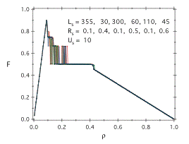
| If we do away with the assumption of two segments only, the model becomes more realistic, but also aquires more paramaters to be determined and the analysis of the model in full parameter ranges become more difficult. We naturally expect, however, that essential characteristics found for two segments model persists with the appearence of the fluctuating third phase. We show on the graph in the right that numerical experiments corroborate this expectation. |
|
This fundamental diagram is obtained from a Nishimura model traffic on a road of L = 1000 cells divided into six segments with a common speed limit U = 10 and with randomely choen lengths Lk with randomely chosen non-accereration rates Rk.
|

