-
First, import
using GLMakie # If you want to display it in a Jupyter notebook, set inline = true # If you want to open a separate window, set inline = false # For interactive, 3D graphs, and animations, inline = false is the default setting GLMakie.activate!(inline = true) # If you want to change font size, or use Japanese set_theme!( fontsize = 32, fonts = (regular = "Noto Sans CJK JP", bold = "Noto Sans CJK JP") ) -
Graph Basics
                # Securing the drawing area
                fig = Figure()

                # Securing the axis
                # fig[1,1] means the graph in the first row and first column
                # Important when arranging multiple graphs (described later)
                ax = Axis(fig[1,1])

                # Draw a line graph on the axis
                # Line graphs are lines! Scatter plots are scatter!
                # If you want to include both dots and lines, use scatterlines!
                lines!(ax, [1;4;7], [2;5;1]) # Line graph connecting (1,2), (4,5), and (7,1)

                # graph drawing
                display(fig)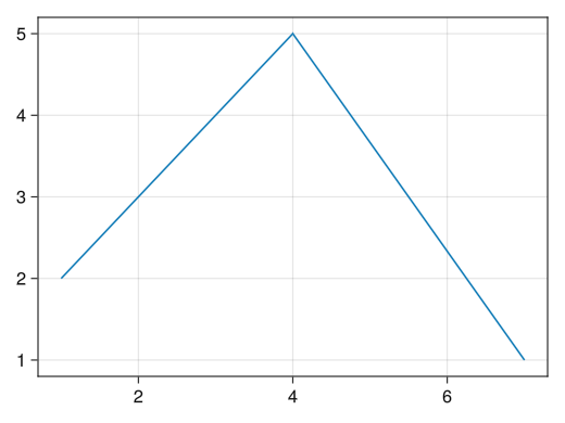
-
Name axes and graphs
                fig = Figure()

                # The xlabel option adds a name to the x-axis
                # The ylabel option adds a name to the y-axis
                # Graphs are named with the title option
                ax = Axis(fig[1,1], xlabel = "Name of the x-axis", ylabel = "Name of the y-axis", title = "Graph of sin(x)")

                x = collect(range(0, 2pi, length = 100))
                lines!(ax, x, sin.(x))

                display(fig)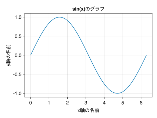
-
Set the axis range
                fig = Figure()

                ax = Axis(fig[1,1], xlabel = "x", ylabel = "sin(x)")

                x = collect(range(0, 2pi, length = 100))
                lines!(ax, x, tan.(x))

                # Specify the range of the x-axis with xlims!
                # Specify the range of the y-axis with ylims!
                # If you want to specify only the upper or lower limit, set the other to nothing
                xlims!(ax, 0, pi)
                ylims!(ax, -5, 5)

                display(fig)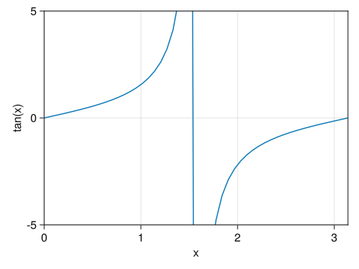
-
Set axis values
                fig = Figure()

                # The xticks! option allows you to specify the numbers to display on the x-axis
                # The yticks! option allows you to specify the numbers to display on the y-axis.
                ax = Axis(fig[1,1], xlabel = "x", ylabel = "sin(x)",
                    xticks = [0; pi/2; pi; 3pi/2; 2pi],
                    yticks = [-1; -0.5; 0; 0.5; 1])

                x = collect(range(0, 2pi, length = 100))
                lines!(ax, x, sin.(x))

                display(fig)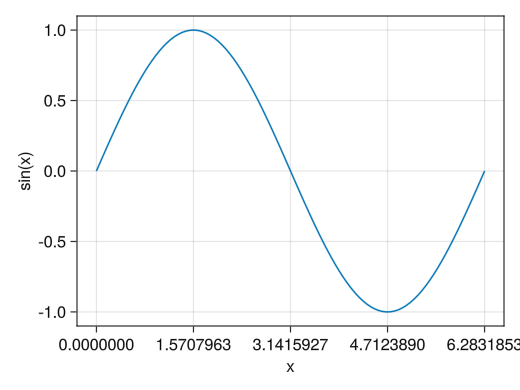
-
Set the values of the axes to whatever notation you want.
                fig = Figure()

                # For x(y)ticks!, by placing two vectors in parentheses
                # You can change the display of specified values
                # The number of elements in the two vectors must be the same
                ax = Axis(fig[1,1], xlabel = "x", ylabel = "sin(x)",
                    xticks = ([0; pi/2; pi; 3pi/2; 2pi], ["0"; "π/2"; "π"; "3π/2"; "2π"]),
                    yticks = ([-1; 0; 1], ["ymin"; "0"; "ymax"]))

                x = collect(range(0, 2pi, length = 100))
                lines!(ax, x, sin.(x))

                display(fig)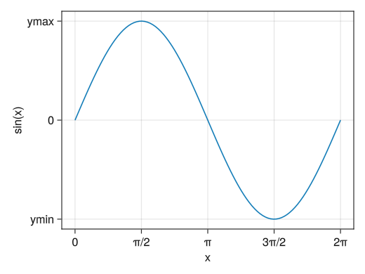
-
Clear the grid
                fig = Figure()

                # x(y)gridvisible = false hides the grid in the x(y) direction
                ax = Axis(fig[1,1], xlabel = "x", ylabel = "sin(x)",
                    xticks = ([0; pi/2; pi; 3pi/2; 2pi], ["0"; "π/2"; "π"; "3π/2"; "2π"]),
                    yticks = ([-1; 0; 1], ["ymin"; "0"; "ymax"]),
                    xgridvisible = false,
                    ygridvisible = false)

                x = collect(range(0, 2pi, length = 100))
                lines!(ax, x, sin.(x))

                display(fig)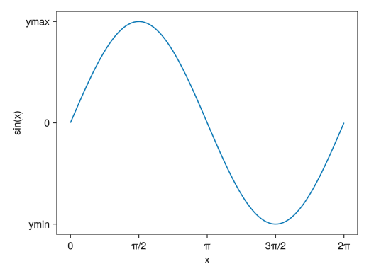
-
Insert a sub-scale with no numerical value
                fig = Figure()

                # x(y)minorticksvisible = true enables the display of sub-ticks in the x(y) direction
                # (Also explained in the logarithmic graph section)
                # You can also specify the specific position of the sub-ticks with the x(y)minorticks option
                # Instead of entering specific values, you can specify the number of sub-ticks between ticks using IntervalsBetween
                ax = Axis(fig[1,1], xlabel = "x", ylabel = "sin(x)",
                    xticks = ([0; pi/2; pi; 3pi/2; 2pi], ["0"; "π/2"; "π"; "3π/2"; "2π"]),
                    yticks = ([-1; 0; 1], ["ymin"; "0"; "ymax"]),
                    xminorticksvisible = true,
                    yminorticksvisible = true)

                x = collect(range(0, 2pi, length = 100))
                lines!(ax, x, sin.(x))

                display(fig)
-
Insert a grid for the sub scale
                fig = Figure()

                # x(y)minorgridvisible = true enables the grid for the x(y) direction sub-ticks (sub-ticks need to be displayed)
                ax = Axis(fig[1,1], xlabel = "x", ylabel = "sin(x)",
                    xticks = ([0; pi/2; pi; 3pi/2; 2pi], ["0"; "π/2"; "π"; "3π/2"; "2π"]),
                    yticks = ([-1; 0; 1], ["ymin"; "0"; "ymax"]),
                    xminorticksvisible = true,
                    yminorticksvisible = true,
                    xminorticks = IntervalsBetween(4),
                    xminorgridvisible = true,
                    yminorgridvisible = true)

                x = collect(range(0, 2pi, length = 100))
                lines!(ax, x, sin.(x))

                display(fig)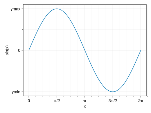
-
Same ratio of length to number on x-axis and y-axis
                fig = Figure()

                # aspect = DataAspect() option sets the ratio of the vertical and horizontal values to be the same
                ax = Axis(fig[1,1], aspect = DataAspect())

                x = collect(range(0, 2pi, length = 100))
                lines!(ax, x, sin.(x))

                display(fig)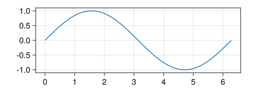
-
Make the x-axis and y-axis have the same length
                fig = Figure()

                # aspect = AxisAspect(1) option makes the vertical and horizontal axes the same length
                ax = Axis(fig[1,1], aspect = AxisAspect(1))

                x = collect(range(0, 2pi, length = 100))
                lines!(ax, x, sin.(x))

                display(fig)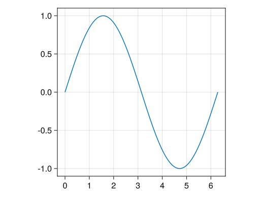
-
Using LaTeX for Strings
                fig = Figure()

                # By adding an L before a string, you can use LaTeX notation
                # However, compared to PythonPlot, the environment is poor, Japanese cannot be used, and fonts cannot be changed
                # It might be better to use special characters (Unicode characters) rather than trying hard with LaTeX
                ax = Axis(fig[1,1], xlabel = L"$x$", ylabel = L"$\sin(x)$",
                    xticks = ([0; pi/2; pi; 3pi/2; 2pi], [L"0"; L"$\pi/2$"; L"$\pi$"; L"$3\pi/2$"; L"$2\pi$"]),
                    yticks = ([-1; 0; 1], [L"$y_\mathrm{min}$"; L"0"; L"$y_\mathrm{max}$"]))

                x = collect(range(0, 2pi, length = 100))
                lines!(ax, x, sin.(x))

                display(fig)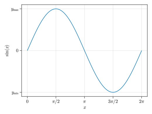
-
Graph Size
                # You can change the size of the drawing area with the resolution option
                # The default size depends on the desktop environment.
                # (Approximately 800 x 600 when operating normally)
                # (Depending on the version, you may be asked to use "size" instead of "resolution," but they are essentially the same)
                fig = Figure(resolution = (400, 300))
                ax = Axis(fig[1,1])
                x = collect(range(0, 2pi, length = 100))
                lines!(ax, x, sin.(x))

                display(fig)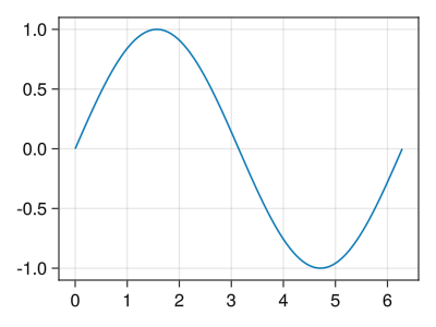
-
Saving Graphs
                fig = Figure()
                ax = Axis(fig[1,1])
                x = collect(range(0, 2pi, length = 100))
                lines!(ax, x, sin.(x))

                # You can save the graph with save("filename", fig)
                # A commonly used file extension is png (automatically determines the file type to save by the file extension)
                # Cannot save as PDF (CairoMakie is required instead of GLMakie)
                save("graph.png", fig)
-
Color, Thickness, Line type
                fig = Figure()
                ax = Axis(fig[1,1])
                x = collect(range(0, 2pi, length = 100))

                # Line width with the linewidth option
                # Line color with color option
                #  :red
                #  (:red, 0.5) : soft red
                # Line type with the linestyle option
                #  :dash
                #  :dot
                #  :dashdot
                lines!(ax, x, sin.(x), linewidth = 4, color = (:violet, 0.5), linestyle = :dashdot)

                display(fig)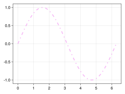
-
Value-based gradient
                fig = Figure()
                ax = Axis(fig[1,1])
                x = collect(range(0, 2pi, length = 100))

                # By specifying a vector for color, a gradient corresponding to the vector value is applied
                lines!(ax, x, sin.(x), color = sin.(x) .^ 2)

                display(fig)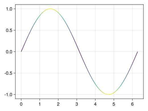
-
Gradient options
                fig = Figure()
                ax = Axis(fig[1,1])
                x = collect(range(0, 2pi, length = 100))

                # Gradation can be changed with the colormap option
                #  :viridis : Common blue→yellow gradient
                #  :jet : rainbow gradient
                #  :hsv : periodic rainbow gradient
                #  :bwr : blue-white-red gradient
                #  :oranges : white→orange gradient
                lines!(ax, x, sin.(x), color = sin.(x) .^ 2, colormap = :jet)

                display(fig)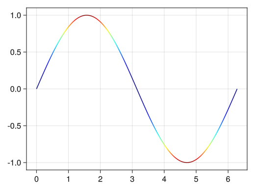
-
Display gradients with color bar
                fig = Figure()
                # Graph in the first row and first column
                ax = Axis(fig[1,1])
                x = collect(range(0, 2pi, length = 100))

                # Assign the line graph itself as a variable (in this case, the variable c_line)
                c_line = lines!(ax, x, sin.(x), color = sin.(x) .^ 2)

                # A color bar for c_line is added to the second row of Colorbar
                Colorbar(fig[1,2], c_line)

                display(fig)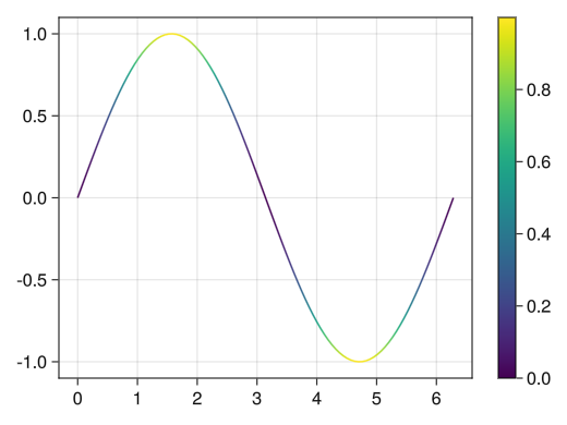
-
Color bar (and gradient) options
                fig = Figure()
                ax = Axis(fig[1,1], xlabel = "x", ylabel = "sin(x)")
                x = collect(range(0, 2pi, length = 100))

                # The colorrange option allows you to set the maximum and minimum values for colors
                c_line = lines!(ax, x, sin.(x), color = sin.(x) .^ 2, colorrange = [0; 1])

                # You can set the scale values with the ticks option
                # Color bars can be named using the label option
                Colorbar(fig[1,2], c_line, ticks = [0; 0.5; 1], label = "sin²(x)")

                display(fig)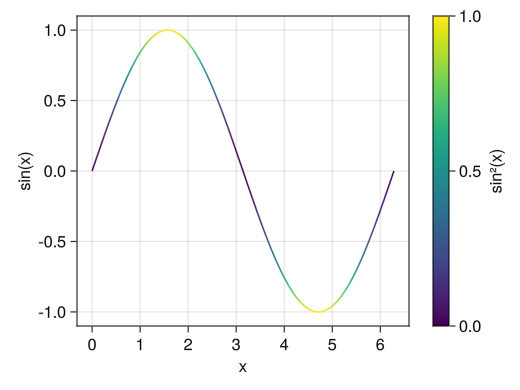
-
Color, Size, Species
                fig = Figure()
                ax = Axis(fig[1,1], xlabel = "height [cm]", ylabel = "weight [kg]")
                height = [172.3; 165; 179.6; 174.5; 173.8; 165.4; 164.5; 174.9; 166.8; 185]
                mass = [75.24; 55.8; 78; 71.1; 67.7; 55.4; 63.7; 77.2; 67.5; 84.6]

                # Point size with the markersize option
                # Point size with the markersize option
                #  :red
                #  (:red, 0.5) : soft red
                # marker options for point types
                #  :circle
                #  :utriangle
                #  :dtriangle
                #  :rect
                scatter!(ax, height, mass, markersize = 25, color = (:blue, 0.5), marker = :rect)

                display(fig)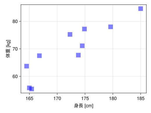
-
Gradient, size, and point type according to value
                fig = Figure()
                ax = Axis(fig[1,1], xlabel = "height [cm]", ylabel = "weight [kg]",
                    title = "Marker size corresponds to age, and scores are based on physical fitness test results")
                height = [172.3; 165; 179.6; 174.5; 173.8; 165.4; 164.5; 174.9; 166.8; 185]
                mass = [75.24; 55.8; 78; 71.1; 67.7; 55.4; 63.7; 77.2; 67.5; 84.6]
                fat = [21.3; 15.7; 20.1; 18.4; 17.1; 22; 32.2; 36.9; 27.6; 14.4]
                age = [27; 25; 31; 32; 28; 36; 42; 33; 54; 28]
                score = ['C'; 'A'; 'C'; 'B'; 'B'; 'B'; 'D'; 'B'; 'C'; 'B']

                # Similar to lines, you can specify a vector for color to create a gradient
                # You can change the size of each point by specifying a vector for markersize
                # You can specify a single character (specified with " instead of ') as a marker to replace the point
                # Furthermore, by specifying a vector, you can change the point type for each point
                c_marker = scatter!(ax, height, mass, markersize = age, color = fat, marker = score)

                # Similar to lines, you can also add color bars to gradients
                Colorbar(fig[1,2], c_marker, label = "body fat [%]")

                display(fig)
-
Draw multiple graphs on a single axis
                fig = Figure()
                ax = Axis(fig[1,1])
                x = collect(range(0, 2pi, length = 100))

                # By repeating lines and scatter, you can draw multiple graphs on a single axis
                # The color changes automatically (of course, you can specify each color individually with the color option)
                lines!(ax, x, sin.(x))
                lines!(ax, x, cos.(x))

                display(fig)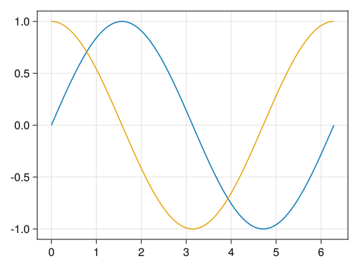
-
Mixed lines and scatter
                fig = Figure()
                ax = Axis(fig[1,1])
                x1 = collect(range(0, 2pi, length = 100))
                x2 = collect(range(0, 2pi, length = 10))
                x3 = collect(range(0, 2pi, length = 15))

                # You can also mix lines, scatter, and scatterlines
                # Please note that color management is separate for lines, scatter, and scatterlines
                lines!(ax, x1, sin.(x1))
                scatter!(ax, x2, cos.(x2))
                scatterlines!(ax, x3, tanh.(x3))

                display(fig)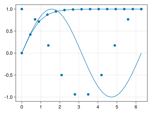
-
Display legend (in graph)
                fig = Figure()
                ax = Axis(fig[1,1], xlabel = "x")
                x1 = collect(range(0, 2pi, length = 100))
                x2 = collect(range(0, 2pi, length = 10))
                x3 = collect(range(0, 2pi, length = 15))

                # Assign the graph itself as a variable
                li = lines!(ax, x1, sin.(x1), color = (:red, 0.5))
                sc = scatter!(ax, x2, cos.(x2), color = (:blue, 0.5))
                sl = scatterlines!(ax, x3, tanh.(x3), color = (:green, 0.5))

                # Display the names assigned with the label option in axislegend as a legend
                axislegend(ax, [li; sc; sl], ["sin(x)"; "cos(x)"; "tanh(x)"])

                display(fig)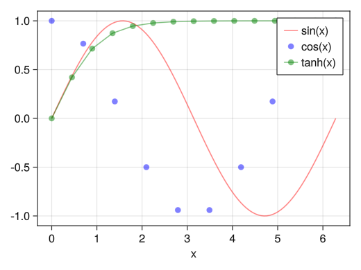
-
Legend Location
                fig = Figure()
                ax = Axis(fig[1,1], xlabel = "x")
                x1 = collect(range(0, 2pi, length = 100))
                x2 = collect(range(0, 2pi, length = 10))
                x3 = collect(range(0, 2pi, length = 15))

                li = lines!(ax, x1, sin.(x1), color = (:red, 0.5))
                sc = scatter!(ax, x2, cos.(x2), color = (:blue, 0.5))
                sl = scatterlines!(ax, x3, tanh.(x3), color = (:green, 0.5))

                # Specify the position with the position option
                #  :rb → right bottom
                #  :rt → right top
                #  :rc → right center
                #  :lb → left bottom
                #  :lt → left top
                #  :lc → left center
                #  :cb → center bottom
                #  :ct → centertop
                #  :cc → center
                axislegend(ax, [li; sc; sl], ["sin(x)"; "cos(x)"; "tanh(x)"], position = :lb)

                display(fig)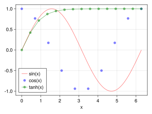
-
Side-by-side legend
                fig = Figure()
                ax = Axis(fig[1,1], xlabel = "x")
                x1 = collect(range(0, 2pi, length = 100))
                x2 = collect(range(0, 2pi, length = 10))
                x3 = collect(range(0, 2pi, length = 15))

                li = lines!(ax, x1, sin.(x1), color = (:red, 0.5))
                sc = scatter!(ax, x2, cos.(x2), color = (:blue, 0.5))
                sl = scatterlines!(ax, x3, tanh.(x3), color = (:green, 0.5))

                # orientationa = :horizontal option makes them appear side by side
                axislegend(ax, [li; sc; sl], ["sin(x)"; "cos(x)"; "tanh(x)"], orientation = :horizontal)

                display(fig)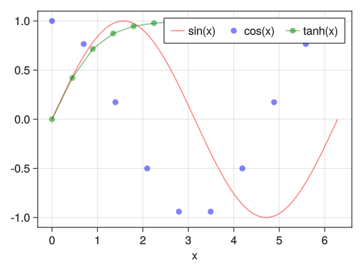
-
Show legend (off graph)
                fig = Figure()
                ax = Axis(fig[1,1], xlabel = "x")
                x1 = collect(range(0, 2pi, length = 100))
                x2 = collect(range(0, 2pi, length = 10))
                x3 = collect(range(0, 2pi, length = 15))

                li = lines!(ax, x1, sin.(x1), color = (:red, 0.5))
                sc = scatter!(ax, x2, cos.(x2), color = (:blue, 0.5))
                sl = scatterlines!(ax, x3, tanh.(x3), color = (:green, 0.5))

                # Displaying legends outside the graph in Legend
                # orientation = :horizontal can also be used
                Legend(fig[1,2], [li; sc; sl], ["sin(x)"; "cos(x)"; "tanh(x)"])

                display(fig)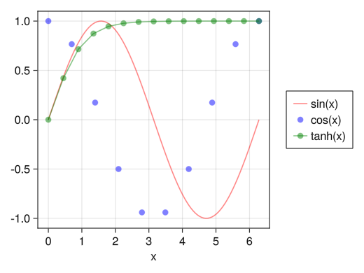
-
Different y-axis for left and right
                fig = Figure()

                ax1 = Axis(fig[1,1], xlabel = "time [s]", ylabel = "velocity [m/s]")

                # yaxisposition = :right enables the right axis as well
                ax2 = Axis(fig[1,1], ylabel = "height [m]", yaxisposition = :right)
                # Add the following two lines as well
                hidespines!(ax2)
                hidexdecorations!(ax2)

                t = collect(range(0, 0.9, length = 100))

                # Please note that color management is separate for ax1 and ax2
                lines!(ax1, t, 5 .- 9.8 * t, color = (:red, 0.5))
                lines!(ax2, t, - 4.9 * t .^ 2 + 5 * t, color = (:blue, 0.5))

                display(fig)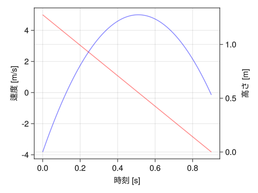
-
Different y-axes for left and right (example with legend)
                fig = Figure(resolution = (720,390))

                ax1 = Axis(fig[1,1], xlabel = "time [s]", ylabel = "velocity [m/s]")
                ax2 = Axis(fig[1,1], ylabel = "height [m]", yaxisposition = :right)
                hidespines!(ax2)
                hidexdecorations!(ax2)

                t = collect(range(0, 0.9, length = 100))

                v0 = lines!(ax1, t, 5 .- 9.8 * t, color = (:red, 0.5))
                vd = lines!(ax1, t, 24.6 * exp.(- t / 2) .- 19.6, color = (:blue, 0.5))
                s0 = lines!(ax2, t, - 4.9 * t .^ 2 + 5 * t, color = (:green, 0.5))
                sd = lines!(ax2, t, 49.2 * (1 .- exp.(- t / 2)) - 19.6 * t, color = (:orange, 0.5))

                Legend(fig[1,2], [v0; vd; s0; sd], ["velocity (without friction) "; "velocity (with friction) "; "height (without friction) "; "height (with friction) "])

                display(fig)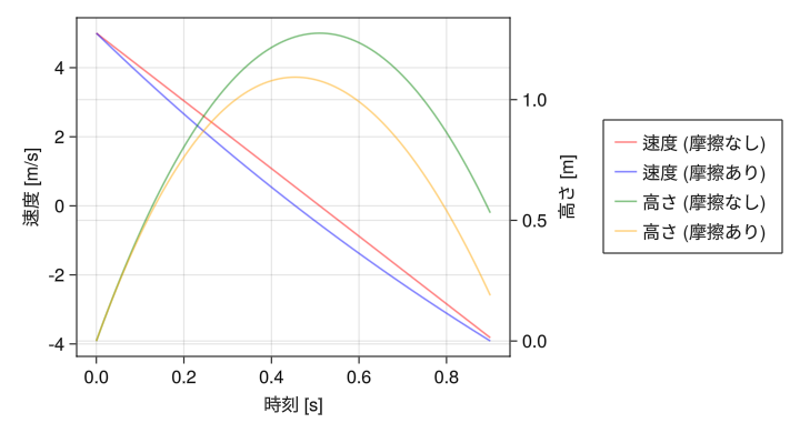
-
Multiple axes
                # Be sure to set the size of the drawing area, as multiple axes will be drawn
                fig = Figure(resolution = (520 * 2 * 0.8, 390 * 3 * 0.8))
                x1 = collect(range(- pi, pi, length = 100))
                x2 = collect(range(-1, 1, length = 100))
                x3 = collect(range(-2, 2, length = 100))
                x4 = collect(range(1, 2, length = 100))

                # Graph in the first row and first column
                ax = Axis(fig[1,1], xlabel = "x", title = "Graph of trigonometric functions")
                li1 = lines!(ax, x1, sin.(x1))
                li2 = lines!(ax, x1, cos.(x1))
                li3 = lines!(ax, x1, tan.(x1))
                ylims!(ax, -1.5, 1.5)
                Legend(fig[1,2], [li1; li2; li3], ["sin(x)"; "cos(x)"; "tan(x)"])

                # Graph in the first row and second column
                ax = Axis(fig[1,3], xlabel = "x", title = "Graph of hyperbolic functions")
                li1 = lines!(ax, x3, sinh.(x3))
                li2 = lines!(ax, x3, cosh.(x3))
                li3 = lines!(ax, x3, tanh.(x3))
                Legend(fig[1,4], [li1; li2; li3], ["sinh(x)"; "cosh(x)"; "tanh(x)"])

                # Graph in the second row and first column
                ax = Axis(fig[2,1], xlabel = "x", title = "Graph of the reciprocal of trigonometric functions")
                li1 = lines!(ax, x1, 1 ./ sin.(x1))
                li2 = lines!(ax, x1, 1 ./ cos.(x1))
                li3 = lines!(ax, x1, 1 ./ tan.(x1))
                ylims!(ax, -10, 10)
                Legend(fig[2,2], [li1; li2; li3], ["csc(x)"; "sec(x)"; "cot(x)"])

                # Graph in the second row and second column
                ax = Axis(fig[2,3], xlabel = "x", title = "Graph of the reciprocal of hyperbolic functions")
                li1 = lines!(ax, x3, 1 ./ sinh.(x3))
                li2 = lines!(ax, x3, 1 ./ cosh.(x3))
                li3 = lines!(ax, x3, 1 ./ tanh.(x3))
                ylims!(ax, -4, 4)
                Legend(fig[2,4], [li1; li2; li3], ["csch(x)"; "sech(x)"; "coth(x)"])

                # Graph in the third row and first column
                ax = Axis(fig[3,1], xlabel = "x", title = "Graph of inverse trigonometric functions")
                li1 = lines!(ax, x2, asin.(x2))
                li2 = lines!(ax, x2, acos.(x2))
                li3 = lines!(ax, x3, atan.(x3))
                Legend(fig[3,2], [li1; li2; li3], ["asin(x)"; "acos(x)"; "atan(x)"])

                # Graph in the third row and second column
                ax = Axis(fig[3,3], xlabel = "x", title = "Graph of inverse hyperbolic functions")
                li1 = lines!(ax, x3, asinh.(x3))
                li2 = lines!(ax, x4, acosh.(x4))
                li3 = lines!(ax, x2, atanh.(x2))
                Legend(fig[3,4], [li1; li2; li3], ["asinh(x)"; "acosh(x)"; "atanh(x)"])

                display(fig)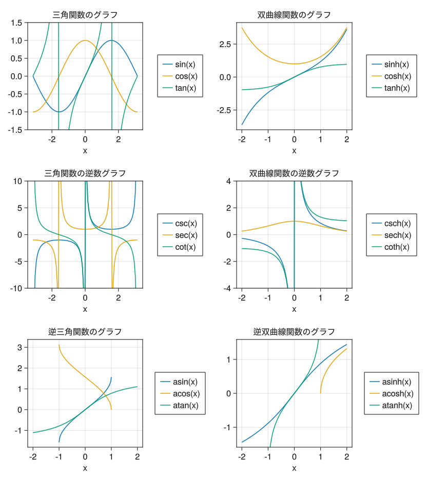
-
single-logarithmic graph
                fig = Figure()

                # yscale = log10 creates a semi-logarithmic graph (y-axis is logarithmic scale)
                ax = Axis(fig[1,1], yscale = log10, xlabel = "x", ylabel = "5 exp(-2x)",
                    title = "In a semi-logarithmic graph, exponential functions appear as straight lines")

                x = collect(range(0, 5, length = 5))
                scatterlines!(ax, x, 5 * exp.(- 2 * x))

                display(fig)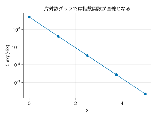
-
double-logarithmic graph
                fig = Figure()

                # Add xscale = log10 to create a double logarithmic graph (logarithmic scale on both the x-axis and y-axis)
                ax = Axis(fig[1,1], xscale = log10, yscale = log10, xlabel = "x", ylabel = "10 x^(-5/3)",
                    title = "In a logarithmic graph, power functions become straight lines")

                x = collect(range(1, 100, length = 10))
                scatterlines!(ax, x, 10 * x .^ (- 5 / 3))

                display(fig)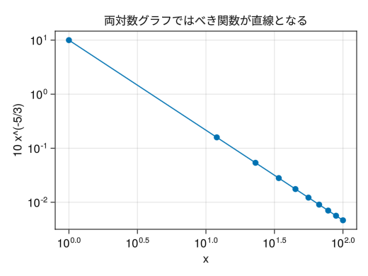
-
Logarithmic graph sub-tick
                fig = Figure()

                # Unlike PythonPlot, sub-ticks are not included by default
                # x(y)minorticksvisible = true to enable minor ticks
                # x(y)minorticks = IntervalBetween specifies the number of minor ticks
                ax = Axis(fig[1,1], xscale = log10, yscale = log10, xlabel = "x", ylabel = "10 x^(-5/3)",
                    title = "In a logarithmic graph, power functions become straight lines",
                    xminorticksvisible = true, yminorticksvisible = true,
                    xminorticks = IntervalsBetween(10), yminorticks = IntervalsBetween(10))

                x = collect(range(1, 100, length = 10))
                scatterlines!(ax, x, 10 * x .^ (- 5 / 3))

                display(fig)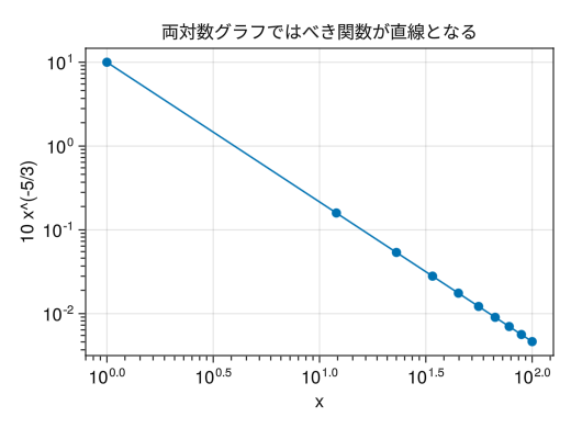
-
Special logarithmic scale
                fig = Figure()

                # Unlike PythonPlot, errors occur when 0 or negative numbers are entered in a logarithmic scale
                # (In the case of PythonPlot, this point is ignored and plotted)
                # As a compromise, a special logarithmic scale, Makie.pseudolog10, is available
                ax = Axis(fig[1,1], yscale = Makie.pseudolog10, xlabel = "x", ylabel = "x³",
                    yticks = [-100; -10; -1; 0; 1; 10; 100])

                x = collect(range(-5, 5, length = 100))
                lines!(ax, x, x .^ 3)

                display(fig)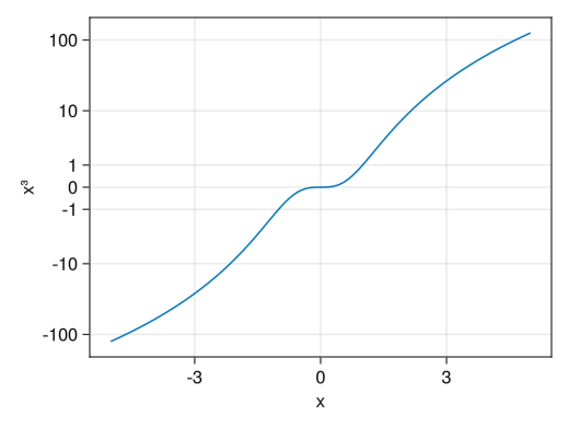
-
Basic histogram
                using Random
                using Dates
                rng = MersenneTwister(Millisecond(now()).value)

                fig = Figure()
                x = [randn(rng, 1000); 2.0 * randn(rng, 1000) .+ 5]

                ax = Axis(fig[1,1], xlabel = "x", ylabel = "頻度")

                # hist!(ax, vector) returns a histogram
                hist!(x)

                display(fig)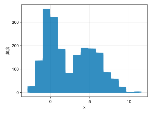
-
change the grade number
                using Random
                using Dates
                rng = MersenneTwister(Millisecond(now()).value)

                fig = Figure()
                x = [randn(rng, 1000); 2.0 * randn(rng, 1000) .+ 5]

                ax = Axis(fig[1,1], xlabel = "x", ylabel = "histogram")

                # Specify the number of classes with the bins option
                hist!(x, bins = 20)

                display(fig)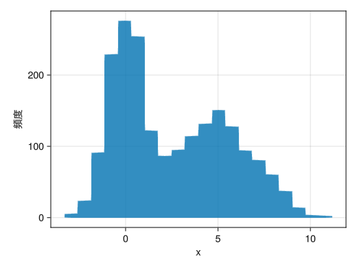
-
Make it a probability distribution, not a frequency
                using Random
                using Dates
                rng = MersenneTwister(Millisecond(now()).value)

                fig = Figure()
                x = [randn(rng, 1000); 2.0 * randn(rng, 1000) .+ 5]

                ax = Axis(fig[1,1], xlabel = "x", ylabel = "p(x)")

                # normalization = :pdf becomes a probability distribution
                hist!(x, bins = 20, normalization = :pdf)

                display(fig)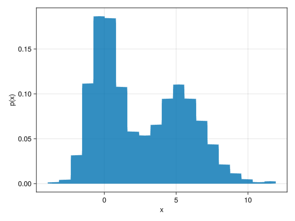
-
Color the outer frame (can this be used to display multiple histograms?)
                using Random
                using Dates
                rng = MersenneTwister(Millisecond(now()).value)

                fig = Figure()
                x1 = randn(rng, 1000)
                x2 = 2.0 * randn(rng, 1000) .+ 5
                x3 = [x1; x2]

                ax = Axis(fig[1,1], xlabel = "x", ylabel = "p(x)")

                # You can specify the outer frame with the strokewidth and strokecolor options
                # Can be used to display multiple histograms simultaneously in combination with color
                h_1 = hist!(x1, bins = 20, normalization = :pdf, color = (:red, 0.05), strokewidth = 1, strokecolor = :red)
                h_2 = hist!(x2, bins = 20, normalization = :pdf, color = (:blue, 0.05), strokewidth = 1, strokecolor = :blue)
                h_3 = hist!(x3, bins = 20, normalization = :pdf, color = (:green, 0.05), strokewidth = 1, strokecolor = :green)

                axislegend(ax, [h1; h2; h3], ["p₁(x)"; "p₂(x)"; "p₁₊₂(x)"])
                display(fig)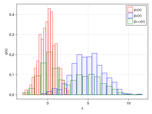
-
A note on histograms
If you want to plot something more advanced, such as a histogram of a line chart, you have to get a vector of the histogram, which can be obtained by the fit function in StatsBase, but it is quite tedious (this is where Python ( numpy) wins hands down).
-
Forced imshow-like heatmap
(not as handy as PythonPlot's imshow)fig = Figure() # Set yreversed = true to reverse the y-axis ax = Axis(fig[1,1], yreversed = true) matrix = [2 3 0 0; 1 2 3 0; 0 1 2 3;] # take the transpose of a matrix # Set interpolate = false to disable interpolation (not necessary for images) # The default is black and white, so specify a color map that is easy to see c_matrix = image!(ax, matrix', interpolate = false, colormap = :viridis) # Color bars can also be added normally Colorbar(fig[1,2], c_matrix) display(fig)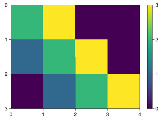
-
Heatmap by heatmap
heatmap is like a contour line, and x and y coordinates can be specified.
The way to specify coordinates is different from PythonPlot's pcolor, which is specified as a vector.
Basically, the line direction of the matrix is x and the column is y.fig = Figure() ax = Axis(fig[1,1], xlabel = "x", ylabel = "y") # Create a vector for the values of x and y x = collect(range(- 2pi, 2pi, length = 100)) y = collect(range(- pi, pi, length = 100)) # heatmap!(ax, vector specifying x coordinates, vector specifying y coordinates, matrix for heat map) # colorrange and colormap options can also be used (see lines) c_heatmap = heatmap!(ax, x, y, sin.(x .+ y')) Colorbar(fig[1,2], c_heatmap, label = "sin(x+y)") display(fig)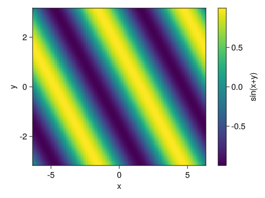
-
In 3D graphs, the viewpoint is changed with the mouse, so it is drawn in a separate window
GLMakie.activate!(inline = false) -
line graph
                fig = Figure()

                # Becomes a 3D graph in Axis3
                # zlabel, zticks, zlims! can be used
                # If you do not want the scale to change automatically when rotating with the mouse, add the viewmode = :fit option (and protrusions = 0 option)
                ax = Axis3(fig[1,1], xlabel = "x = sin(t)", ylabel = "y = cos(t)", zlabel = "z = t + sin(2t)")

                t = collect(range(0, 2pi, length = 100))
                x = sin.(t)
                y = cos.(t)
                z = t + sin.(2t)

                # lines!(ax, x vector, y vector, z vector) creates a line graph
                lines!(ax, x, y, z)

                display(fig)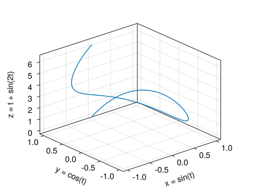
-
Dispersal Chart
                fig = Figure()

                ax = Axis3(fig[1,1], xlabel = "height [cm]", ylabel = "weight [kg]", zlabel = "blood pressure [mmHg]",
                    title = "Marker size corresponds to age, and scores are based on physical fitness test results")
                height = [172.3; 165; 179.6; 174.5; 173.8; 165.4; 164.5; 174.9; 166.8; 185]
                mass = [75.24; 55.8; 78; 71.1; 67.7; 55.4; 63.7; 77.2; 67.5; 84.6]
                blood = [130; 126; 152; 147; 127; 119; 135; 137; 165; 156]
                fat = [21.3; 15.7; 20.1; 18.4; 17.1; 22; 32.2; 36.9; 27.6; 14.4]
                age = [27; 25; 31; 32; 28; 36; 42; 33; 54; 28]
                score = ['C'; 'A'; 'C'; 'B'; 'B'; 'B'; 'D'; 'B'; 'C'; 'B']

                # scatter!(ax, x vector, y vector, z vector) creates a dispersal chart
                c_marker = scatter!(ax, height, mass, blood, markersize = age, color = fat, marker = score)

                Colorbar(fig[1,2], c_marker, label = "body fat [%]")

                display(fig)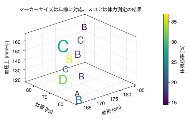
-
Wireframe (display that changes to heatmap)
                fig = Figure()
                ax = Axis3(fig[1,1], xlabel = "x", ylabel = "y", zlabel = "sin(x+y)")

                x = collect(range(- 2pi, 2pi, length = 20))
                y = collect(range(- pi, pi, length = 20))

                # wireframe!(ax, vector specifying x-coordinate, vector specifying y-coordinate, matrix for wireframe)
                wireframe!(ax, x, y, sin.(x .+ y'))

                display(fig)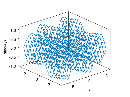
-
Colored surface
                fig = Figure()
                ax = Axis3(fig[1,1], xlabel = "x", ylabel = "y", zlabel = "sin(x+y)")

                x = collect(range(- 2pi, 2pi, length = 100))
                y = collect(range(- pi, pi, length = 100))

                surface!(ax, x, y, sin.(x .+ y'))

                display(fig)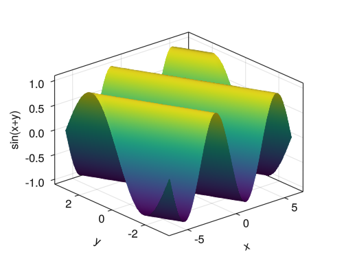
-
Colored surfaces (z values correspond to different colors)
                fig = Figure()
                ax = Axis3(fig[1,1], xlabel = "x", ylabel = "y", zlabel = "tanh(r)")

                x = collect(range(- 5, 5, length = 100))
                y = collect(range(- 5, 5, length = 100))
                r = sqrt.(x .^2 .+ y' .^ 2)
                θ = atan.(0 * x .+ y', x .+ 0 * y')

                # color = Color for the matrix in the matrix
                c_surface = surface!(ax, x, y, tanh(r), color = θ, colorrange = [-pi; pi])

                Colorbar(fig[1,2], c_surface, label = "θ", ticks = ([-pi; 0; pi], ["-π"; "0"; "π"]))

                display(fig)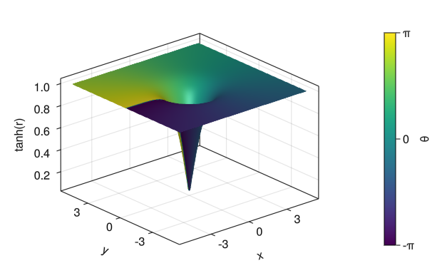
-
Interactive graphs use sliders to change parameters, so they are drawn in a separate window
GLMakie.activate!(inline = false) -
Change parameters in real time using sliders
fig = Figure() ax = Axis(fig[1,1], xlabel = "time [sec]", ylabel = "height") xlims!(ax, 0, 1) ylims!(ax, 0, 1.4) t = collect(range(0, 1, length = 100)) # Create a slider # Basic information about sliders in SliderGrid slider_base = SliderGrid( fig[2,1], # slider location # Enter the number of sliders you want to create in parentheses, followed by a comma # label for name, range for range, startvalue for initial value (label = "initial velocity [m/s]", range = 0:0.1:5, startvalue = 5), (label = "friction [/sec]", range = 0.1:0.1:2, startvalue = 0.1), ) # Read data from basic slider information # Basically, you can just copy and paste here slider_value = [s.value for s in slider_base.sliders] # Creating vectors from slider data S0 = lift(slider_value...) do slider_params... v0 = slider_params[1] - 4.9 * t .^ 2 + v0 * t end Se = lift(slider_value...) do slider_params... v0 = slider_params[1] e = slider_params[2] (9.8 + e * v0) * (1 .- exp.(- e * t)) / e^2 - 9.8 * t / e end S0_line = lines!(ax, t, S0) Se_line = lines!(ax, t, Se) axislegend(ax, [S0_line, Se_line], ["without friction", "with friction"]) display(fig) -
Handling Observable with @list
Vectors S0 and Se in the example above are variables of type Observable that reflect the slider data in real time.
Functions on Observable variables and reading them with title, xlim, etc. The function @lift is necessary to read in Observable variables with a function, title, xlim, etc.fig = Figure() ax = Axis(fig[1,1], xlabel = "time [sec]", ylabel = "height") t = collect(range(0, 2, length = 100)) slider_base = SliderGrid( fig[2,1], (label = "initial velocity [m/s]", range = 1:0.1:10, startvalue = 2), (label = "friction [/sec]", range = 0.1:0.1:2, startvalue = 2), ) slider_value = [s.value for s in slider_base.sliders] S0 = lift(slider_value...) do slider_params... v0 = slider_params[1] - 4.9 * t .^ 2 + v0 * t end Se = lift(slider_value...) do slider_params... v0 = slider_params[1] e = slider_params[2] (9.8 + e * v0) * (1 .- exp.(- e * t)) / e^2 - 9.8 * t / e end # The next value tmax is also an Observable variable tmax = lift(slider_value...) do slider_params... v0 = slider_params[1] v0 / 4.9 end S0_line = lines!(ax, t, S0) Se_line = lines!(ax, t, Se) axislegend(ax, [S0_line, Se_line], ["without friction", "with friction"]) # Put $ before observable variables @lift(xlims!(ax, 0, $tmax)) @lift(ylims!(ax, 0, maximum($S0))) display(fig)
-
Animation is drawn in a separate window
GLMakie.activate!(inline = false) -
The animation is created in the manner of a so-called flipbook.
However, unlike PythonPlot, the animation is created by plotting the function of an Observable variable
and updating that variable, rather than recreating the graphfig = Figure() q = pi / 4 v0 = 5.0 v0x = v0 * cos(q) v0y = v0 * sin(q) g = 9.8 t = 0.0 x = 0.0 y = 0.0 # Create Observable variables for t, x, and y (t is a string) t_obs = Observable(string(t)) x_obs = Observable(x) y_obs = Observable(y) # Operations containing observable variables require @lift # (See interactive graph) ax = Axis(fig[1,1], xlabel = "horizontal distance [m]", ylabel = "vertical distance [m]", title = @lift("t = " * $t_obs * " [sec]")) # graph plot scatter!(ax, x_obs, y_obs) xlims!(ax, 0, 3) ylims!(ax, 0, 0.8) display(fig) # For loop to display animation for it = 1:200 t = it * 0.0035 x = v0x * t y = v0y * t - 0.5 * g * t ^ 2 # Stop calculations for a specified time (seconds) before updating observable variables sleep(0.05) # Updating observable variables t_obs[] = string(t) x_obs[] = x y_obs[] = y end -
A few tips
using Printf fig = Figure() q = pi / 4 v0 = 5.0 v0x = v0 * cos(q) v0y = v0 * sin(q) g = 9.8 t = 0.0 x = 0.0 y = 0.0 # Vector for plotting point trajectories # Start by setting all elements to NaN (undefined value). xt = zeros(200) * NaN yt = zeros(200) * NaN # You can specify the number of significant digits using @sprintf. 5.3f means that three digits after the decimal point are displayed using five spaces # (Requires the Printf library) t_obs = Observable(@sprintf("%5.3f", t)) x_obs = Observable(x) y_obs = Observable(y) xt_obs = Observable(xt) yt_obs = Observable(yt) ax = Axis(fig[1,1], xlabel = "horizontal distance [m]", ylabel = "vertical distance [m]", title = @lift("t = " * $t_obs * " [sec]")) scatter!(ax, x_obs, y_obs) lines!(ax, xt_obs, yt_obs) xlims!(ax, 0, 3) ylims!(ax, 0, 0.8) display(fig) for it = 1:200 t = it * 0.0035 x = v0x * t y = v0y * t - 0.5 * g * t ^ 2 xt[it] = x yt[it] = y sleep(0.05) t_obs[] = @sprintf("%5.3f", t) x_obs[] = x y_obs[] = y xt_obs[] = xt yt_obs[] = yt end -
Save animation
                fig = Figure()

                q = pi / 4
                v0 = 5.0
                v0x = v0 * cos(q)
                v0y = v0 * sin(q)
                g = 9.8

                t = 0.0
                x = 0.0
                y = 0.0

                xt = zeros(200) * NaN
                yt = zeros(200) * NaN

                t_obs = Observable(@sprintf("%5.3f", t))
                t_obs = Observable(t)
                x_obs = Observable(x)
                y_obs = Observable(y)
                xt_obs = Observable(xt)
                yt_obs = Observable(yt)

                ax = Axis(fig[1,1], xlabel = "horizontal distance [m]", ylabel = "vertical distance [m]",
                    title = @lift("t = " * $t_obs * " [sec]"))

                scatter!(ax, x_obs, y_obs)
                lines!(ax, xt_obs, yt_obs)
                xlims!(ax, 0, 3)
                ylims!(ax, 0, 0.8)

                # Use record instead of for to save animations
                record(fig, "animation.mp4", 1:200, framerate = 20) do it

                    # If you leave display(fig) here, you can check the animation.
                    display(fig)

                    t = it * 0.0035
                    x = v0x * t
                    y = v0y * t - 0.5 * g * t ^ 2
                    xt[it] = x
                    yt[it] = y

                    sleep(0.05)

                    t_obs[] = @sprintf("%5.3f", t)
                    x_obs[] = x
                    y_obs[] = y
                    xt_obs[] = xt
                    yt_obs[] = yt
                end